Fetching Road Data with `fetch_roads()`

This vignette demonstrates how to use the fetch_roads() function to download road data from OpenStreetMap (OSM). You can fetch data for a specific area using either a bounding box or a center point with a radius, and optionally crop the data to the precise boundaries.

Fetching by bounding box

This example is to specify a rectangular area using a bounding box. By default, fetch_roads() returns all roads that intersect the box. Setting crop = TRUE will trim the to the box’s boundaries.

# Define a bounding box (e.g., around Sakae area, Japan)
sakae_bbox <- create_bbox(north =  35.17377,
                          south =  35.16377,
                          east  = 136.91590,
                          west  = 136.90090)

# 1. Fetch roads without cropping (default)
roads_default <- fetch_roads(sakae_bbox)
plot(roads_default$geometry, lwd = 2)
plot(convert_bbox_to_polygon(sakae_bbox), add = TRUE, border = "red", lty = 2, lwd = 2)

# 2. Fetch roads with cropping
roads_cropped <- fetch_roads(sakae_bbox, crop = TRUE)
plot(roads_cropped$geometry, lwd = 2)
plot(convert_bbox_to_polygon(sakae_bbox), add = TRUE, border = "red", lty = 2, lwd = 2)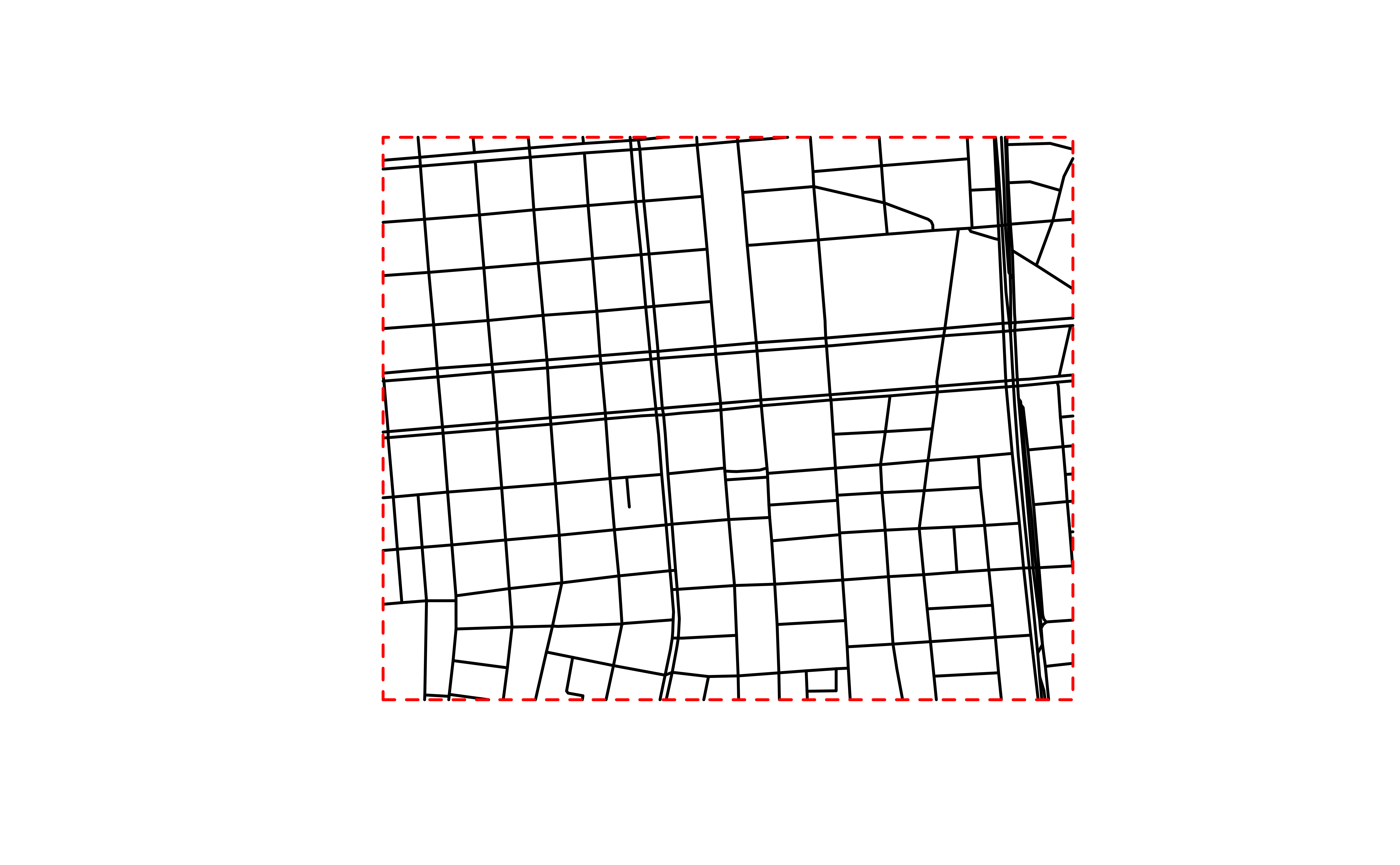

As shown in the plots, crop = TRUE trims the road geometries precisely to the red-dashed boundary.

Fetching by center point and radius

You can specify a center point (longitude and latitude) and a search radius in meters. To get roads trimmed to the circular area, you must set both crop = TRUE and cricle_crop = TRUE

# Define a center point (Nagoya Station) and radius
center_lon <- 136.8817
center_lat <-  35.1709
radius_m   <- 500

# Fetch and crop roads to a circular area
roads_circle_cropped <- fetch_roads(x           = center_lon,
                                    y           = center_lat,
                                    radius      = radius_m,
                                    crop        = TRUE,
                                    circle_crop = TRUE)


# Plot the result
plot(roads_circle_cropped$geometry, lwd = 2)

# Draw the circle boundary for visualization
center_pt   <- create_points(center_lon, center_lat, crs = 4326)
circle_poly <- st_buffer(transform_to_cartesian(center_pt), radius_m)
plot(transform_to_geographic(circle_poly), add = TRUE, border = "red", lty = 2, lwd = 2)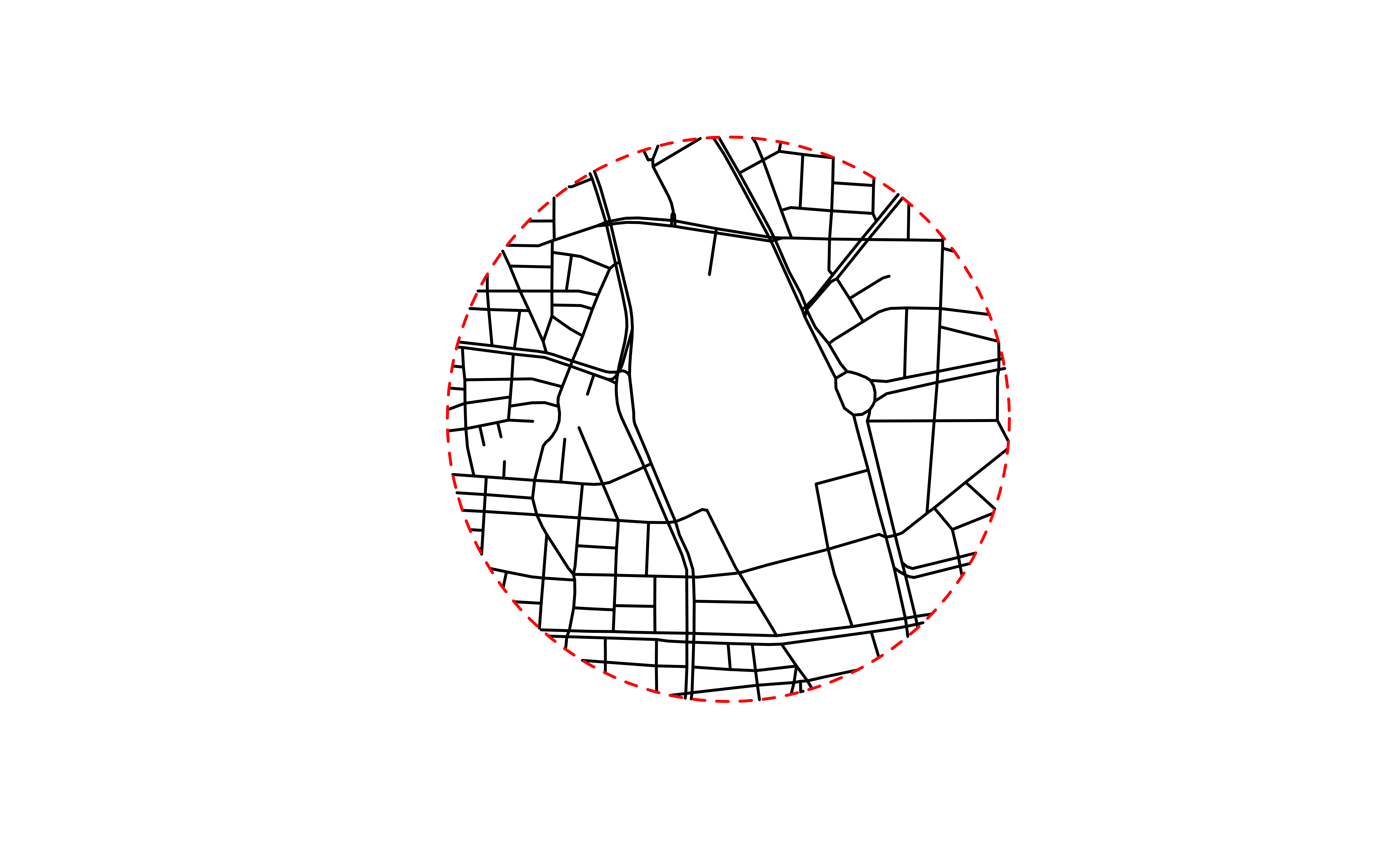

The plot shows that the road network is perfectly contained within the specified circular boundary.