Plot spatiotemporal network or TNKDE results

Creates a plot to visualize the events, counts, or TNKDE density on a spatiotemporal network. The default is a 2D snapshot plot. The 3D view is optimized for visualizing TNKDE results across time.

Usage

# S3 method for class 'spatiotemporal_network'
plot(
  x,
  y,
  mode = c("event", "count", "density"),
  snapshot_time = 12,
  plot_3d = FALSE,
  time_range = 0:23,
  ...
)

Arguments

x

The spatiotemporal_network object (often the output of convolute_spatiotemporal_network).

y

(Not used).

mode

Character string specifying the type of visualization: "event" (individual points), "count" (event count per segment), or "density" (TNKDE density).

snapshot_time

Numeric. The hour (0-23) for which to create the static 2D snapshot plot.

plot_3d

Logical. If TRUE, an interactive 3D plot using rgl is created.

time_range

Numeric vector (e.g., 0:23) specifying the time points to include in the 3D plot.

...

Additional arguments passed to helper functions.

Value

NULL (invisibly). Opens an interactive rgl window for 3D plots, or draws a base R plot for 2D.

Examples

# Run the TNKDE calculation
tnkde_result <- sample_roads |>
  create_road_network() |>
  create_spatiotemporal_network(
    spatial_length = 0.5,
    temporal_length = "1 hour"
  ) |>
  set_events(sample_accidents, time_column = "time") |>
  convolute_spatiotemporal_network(
    bandwidth_space = 2,
    bandwidth_time = 1.5,
    time_points = 0:23
  )

# Plotting examples:

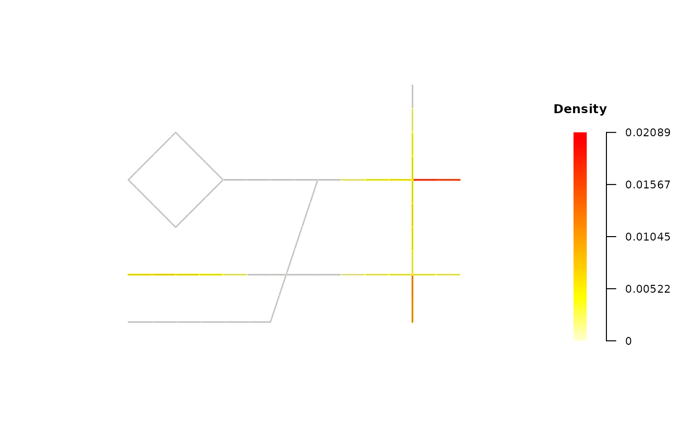
# A. 2D Snapshot: smoothed density
# Use Case: Visualize the primary analysis result at 19:00.
plot(tnkde_result, mode = "density", snapshot_time = 19)


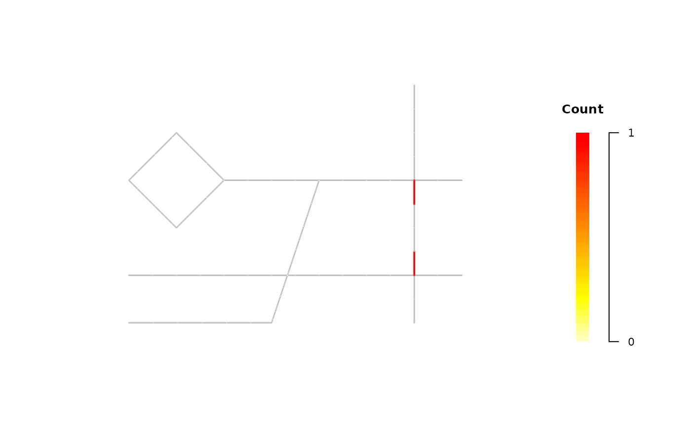
# B. 2D Snapshot: raw event counts per segment
# Use Case: See raw event counts at a specific hour (e.g., 7:00).
plot(tnkde_result, mode = "count", snapshot_time = 7)


# C. 3D Plot: full density cube
# This is the primary visualization for spatiotemporal analysis.
# plot(tnkde_result, mode = "density", plot_3d = TRUE)